English


Discounts for lack of marketability (DLOMs) have frequently been the subject of controversy in valuations. The reason: applying a DLOM – an amount or percentage deducted from the value of an ownership interest to reflect the relative absence of marketability – can result in significant value reduction compared with the pro rata value of a business interest. Today’s valuation practitioners use numerous methods1 that can be classified into four main categories, each with its advantages and disadvantages:
- Benchmark study: utilizes restricted stocks and initial public offering pricing data
- Security-based approach: utilizes theoretical option pricing models, illiquidity estimates demonstrated by traded stock prices, and option prices
- Analytics: utilizes historical studies on private placement of equity
- Other approaches: Quantitative Marketability Discount Model (QMDM), Nonmarketable Investment Company Evaluation (NICE), etc.
In analyzing data sets, several key weaknesses become evident: the demonstration of a selection bias (i.e., picking data based on availability); the introduction of subjective inputs; and references to outdated data, disparate standards, and periods of significant change. Finally, results derived from data set analysis can lead to wide ranges of DLOMs that require a qualitative assessment in order to conclude specific value.
Based on this understanding, and on empirical evidence after implementing various techniques, the implementation of option pricing models has been identified as the most appropriate method for estimating DLOMs.2 This article describes the four principal models of this type:
- Chaffe: Black-Scholes-Merton put option
- Longstaff: lookback put option
- Finnerty: average-strike put option
- Ghaidarov: average-strike put option
The article then presents a simple case study and outlines a useful framework for valuing interests in private companies using an efficient, effective quantitative model.
Option Pricing Models
David Chaffe, in his 1993 option pricing study, highlighted a link between a DLOM and the cost to purchase a European put option.3 Chaffe’s theory was as follows:
If one holds restricted or nonmarketable stock and purchases an option to sell those shares at the free market price, the holder has, in effect, purchased marketability for those shares. The price of this put is the discount for lack of marketability.
Because Chaffe relied on the Black-Scholes-Merton put option pricing model, the inputs to his model are the stock price, the strike price, the time to expiration, the interest rate, and volatility. In the Chaffe model, the stock price and the strike price equal the marketable value of the private company stock as of the valuation date. Due to its reliance on European options, the Chaffe model is downward-biased. Consequently, the results derived by his model should be considered a lower bound for estimating DLOMs.
Francis Longstaff, meanwhile, used a lookback put option – an exotic option with path dependency – to estimate DLOMs.4 In this case, the payoff depends on the optimal price of the underlying asset occurring over the life of the option. The options allow the holder to “look back” over time to determine the payoff. Yet the Longstaff model assumes that an investor has perfect market timing and, as a result, reflects an upper bound for DLOMs. Finally, there is disagreement over whether the Longstaff model concludes to a DLOM or to a liquidity premium that needs to be converted to a discount.
John Finnerty extended Longstaff’s work by utilizing an average-strike put option that is also exotic but does not assume perfect market timing.5 The Finnerty model appears to work very well at lower volatilities, but yields low DLOMs at higher volatilities when compared with the restricted stock transactions. Furthermore, because it yielded DLOMs that exceeded 100%, the original Finnerty model had to be revised. The revised model produces no discount in excess of 32.3%, regardless of higher volatilities and longer holding times. This limitation may significantly understate the DLOM for volatilities exceeding 125% and six-month holding horizons. These inputs are relatively rare in valuations, however.
Like Finnerty, Stillian Ghaidarov also uses average-strike put options.6 The results of the Ghaidarov model – developed as a criticism to the original Finnerty model – closely match the modified Finnerty model for the sixmonth holding period and volatilities through 125%. Past this point though, the Ghaidarov model can generate DLOMs that are significantly higher than the results indicated by restricted share studies. These should be used with caution.
Overall, based on our experience in the respective inputs to these models, their levels of difficulty, and the generated estimates for different asset classes, we believe that the Finnerty model is the most appropriate method to estimate DLOMs for financial reporting purposes. It is worth mentioning, though, that for tax-related valuation purposes, the Stout Restricted Stock Study™ (formerly the FMV Restricted Stock Study) is a more relevant valuation tool.
Framework: Sample Case
The discount associated with the illiquidity of each type of instrument included in a capital structure of a private company is directly related to its inherent rights and privileges. In each case, the level of discount applicable depends on a number of parameters, including the instrument’s overall seniority in a capital structure; whether it is considered to be in the money, at the money, or out of the money as of the measurement date (with regard to the corresponding participation thresholds); the level of equity volatility used for valuation purposes; the effective time frame for the analysis; and the company’s dividend policy. From a valuation perspective, securities with higher seniority or more protective provisions are associated with a lower illiquidity discount due to the lower risk of receiving distributions below certain thresholds or beyond certain time frames expected by potential investors. On the other hand, securities that are very junior in capital structures – and thus lack any substantial control over the company’s operating and managerial decisions – translate to a higher illiquidity discount due to the higher risks associated with achieving the expected returns over the holding period.
When measuring the appropriate illiquidity discount in complex capital structures, one crucial complexity involves the search for a quantitative and qualitative way to differentiate the applicable discount among the various securities analyzed. This article relies on the framework introduced by Dwight Grant in “Thoughts on Calculating DLOMS,” where the discount applicable in a random security is positively correlated to the volatility of the specified security within the framework of the given capital structure under examination.7 The first step in calculating the appropriate volatility of a security included in a given capital structure is to develop a Black-Scholes option pricing model (BSOPM): an arbitrage pricing model developed using the premise that two assets with identical payoffs must have identical prices to prevent arbitrage. The BSOPM, which relies on such variables as asset price, strike price, expected term, risk-free rate, volatility, and dividend yield, is basically a contingent claim analysis that treats equity as a combination of call options associated with the claims of each security included in the capital structure. The strike prices of these options correspond to the participation thresholds of these securities, and the respective call options represent the value attributable to these securities above the specified strike prices (or breakpoints) based on the set of required assumptions.
After calculating the values of the call options, the next step is to calculate the delta that corresponds to each security. The delta measures the changes in the value of the call options relative to the change in the value of the asset price – in this case, the equity value of the company. In other words, the delta measures the relationship between the volatility of the equity value and the value of the specific security, which is considered to be a derivative instrument on the equity value of the company. The delta spreads of the different call options are used to estimate the aggregate delta associated with each security class, which is equal to the sum of each security class’ ownership claim on the calculated delta spreads. The volatility for each security class can then be expressed as the product of the aggregate delta, the leverage ratio (based on the underlying asset price relative to the total claims of each security class), and the assumed equity volatility. Based on the concluded asset volatility for each security, the appropriate DLOM is finally calculated based on the revised Finnerty model.
Below, we present a simple case with a hypothetical capital structure that includes only one type each of preferred security, common units, and options on common stock. Figure 1 shows a summary of the assumed capital structure.
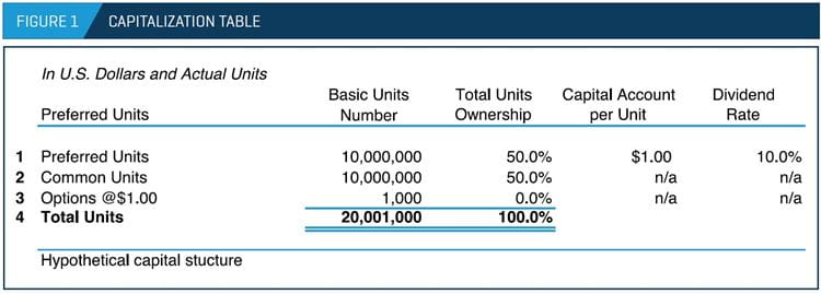
Figure 2 presents the BSOPM framework vis-à-vis the rights and privileges of the securities analyzed, based on the assumed capital structure.
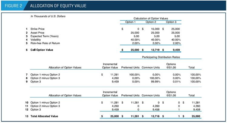
Figure 3 presents both the individual security volatility analysis and the calculation of the appropriate DLOM applicable to each security.
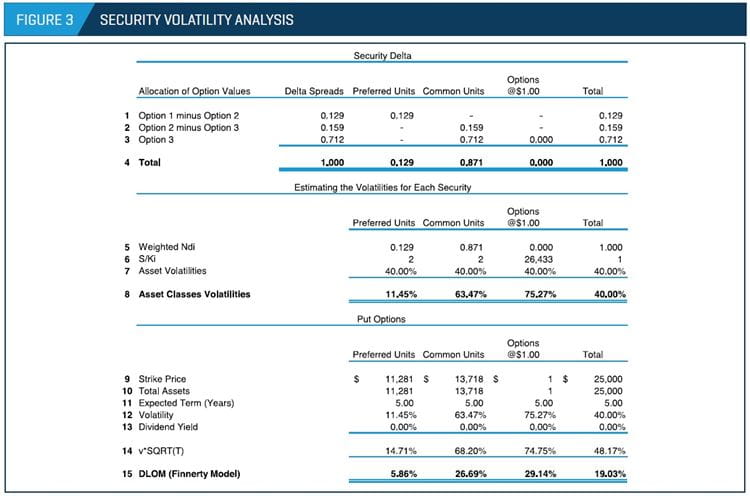
As presented in line 8 (in Figure 3), the concluded asset volatility is lower for the most senior securities and higher for the more junior securities – a reasonable conclusion based on the expectations described earlier. The same relationship is observed between the seniority of the securities and the concluded DLOM based on the Finnerty model, which relies on the concluded asset volatility for each security along with the assumptions for the expected holding term and the dividend yield. The preferred units, which enjoy greater seniority in the capital structure, are subject to a lower illiquidity discount compared with lower seniority attributed to the “options @$1.00.” The difference between the concluded illiquidity discounts of these securities might increase or decrease based on the set of assumptions used for the purpose of the BSOPM analysis.
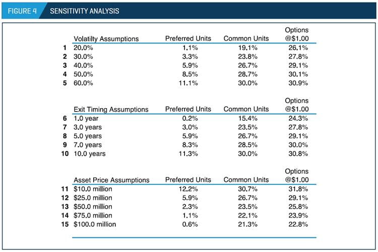
Figure 4 presents a sensitivity analysis based on different volatility, exit timing, and asset price assumptions, and on the impact on the concluded DLOM among the different securities. Figure 4 reveals a positive relationship between the volatility or holding period assumption and the concluded DLOM. Higher volatility or holding period assumptions lead to higher applicable illiquidity discounts due to the greater uncertainty and risk concerning future realized distribution levels. The opposite relationship can be observed concerning the applicable asset price allocated: higher asset price inputs produce lower illiquidity discounts because of the lower risk associated with the probability of the analyzed securities being out of the money at the end of the holding period.
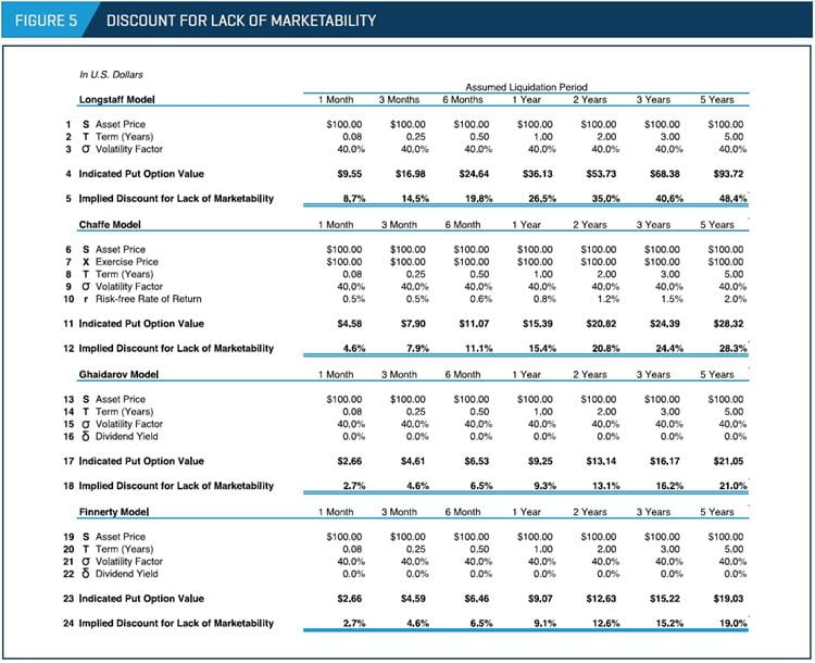
Finally, Figure 5 presents the results of the different quantitative methods described earlier, based on different holding periods and an assumed volatility of 40%.
Consider Both Quantitative and Qualitative Provisions
The framework outlined here is an expedient tool for valuing interests in private companies with a quantitative model that differentiates securities and assigns different illiquidity discounts based on their relative rights and privileges (and on the remaining assumptions linked to the BSOPM framework and management inputs). However, qualitative factors associated with ownership control premiums, voting rights, or other protective provisions should always be considered in order to avoid determining an illiquidity discount that over- or understates the value of the subject interest.
- IRS. Discount for Lack of Marketability: Job Aid for IRS Valuation Professionals. September 2009.
- Aaron Rotkowski and Michael Harter, “Current Controversies Regarding Option Pricing Models,” Taxation Planning and Compliance Insights, Autumn 2013.
- David Chaffe, “Option Pricing as a Proxy for Discount for Lack of Marketability in Private Company Valuations.” Business Valuation Review, 12, 4:182-188, 1993.
- John Elmore, “Determining the Discount for Lack of Marketability with Put Option Pricing Models in View of the Section 2704 Proposed Regulations.” Valuation Practices and Procedures Insights, Winter 2017.
- John D. Finnerty, “An Average-Strike Put Option Model of Marketability Discount.” The Journal of Derivatives, 19, 4:53-69, 2012.
- Stillian Ghaidarov, ‘‘The Use of Protective Put Options in Quantifying Marketability Discounts Applicable to Common and Preferred Interests.’’ Business Valuation Review, 28, 2:88-99, 2009.
- Dwight Grant, “Thoughts on Calculating DLOMs,” Business Valuation Review, 33, 4:102-112, 2014.