English


In 2019, the oil and gas industry experienced a decline in total deal value and volume compared with 2018. The exploration and production (E&P) segment accounted for the majority of the deal activity in 2019. The decrease in deal activity was largely the result of investor and bank pessimism, which has limited E&P companies’ access to capital markets and has forced them to live within their cash flows. Despite the overall decrease in deal activity, as in previous years, the number of property-related transactions exceeded the number of corporate transactions. We explore some of the inputs in projecting cash flow for oil and gas properties after an acquisition either internally for corporate budgeting purposes or when used in valuations performed under fair value accounting.
In both cases, determining the expected annual free cash flow associated with the acquired properties is critical. However, many factors must be considered when calculating the free cash flow associated with such oil and gas properties.
Stock vs. Asset Transaction
Before projecting oil and gas cash flow for acquired properties, analysts should first determine how the transaction was structured. An acquisition can be structured as an asset transaction or as a stock transaction. An asset transaction involves the sale of individual assets and liabilities; a stock transaction involves the sale of the owner’s or owners’ shares in the overall business. Typically, the purchase of oil and gas properties is structured as an asset transaction, so the buyer can step up the basis of the assets to fair value and increase certain tax deductions.[1]
Oil and Gas Revenue
There are many ways to estimate and project oil and gas revenue. An analyst can utilize a reserve report prepared by a petroleum engineer or can estimate oil and gas revenue based on their own assumptions. The first step in estimating the revenue for the acquired oil and gas properties is estimating the annual volumes of oil and gas that could be produced from the properties.[2] Ideally, with the help of a petroleum engineer, analysts can develop a decline curve analysis. A decline curve analysis involves predicting future oil well or gas well production based on the production history. Many variables go into determining the estimated production volumes of oil and gas that can be produced: the geology of the sub-surface, the number of wells assumed, the well spacing, the production decline rate, the results from neighboring properties, etc. Based on these factors, the petroleum engineer can estimate the annual barrels of oil and cubic feet of natural gas that can be produced from the acquired properties.
The next step in estimating the revenue for oil and gas properties is determining the appropriate commodity prices. For fair value accounting purposes, it is customary to use futures prices of oil and natural gas, as of the transaction date, as traded on the New York Mercantile Exchange, or NYMEX pricing. For internal purposes, analysts can use their own estimation of future prices. Stout typically uses three years of NYMEX prices and then escalates them based on inflation.[3] In some cases, firms have been known to use the full five years of NYMEX prices and then inflate these prices for a finite period before keeping prices flat for the remainder of the projection period. Once analysts have their estimated commodities prices, they then adjust the prices for estimated differentials based on historical differences between NYMEX prices and the actual prices realized by the acquired properties. These adjust¬ments reflect differences in heating value, quality, gravity, and other factors, as well as the associated transportation costs.
Once analysts have determined the realized prices and the estimated volumes, they can estimate the oil and gas revenue of the acquired properties by multiplying the volumes by the estimated realized prices.
Operating Cash Flow
The operating cash flow of the acquired properties is determined by subtracting severance taxes, ad valorem taxes, operating costs, and abandonment cost from the oil and gas revenue.
Severance taxes are taxes charged to producers, or anyone with a working or royalty interest in oil, gas, or mineral operations. Most states levy a severance tax when oil and gas are produced in the state. The tax is calculated based on either the value or the volume of production, although sometimes states use a combination. This tax is generally levied at the time and place the minerals are severed from the producing reservoir, as the name implies. To estimate severance taxes, the tax rate is multiplied by the oil and gas revenue.
Ad valorem taxes are essentially property taxes. They are levied by counties based on the appraised value of the oil and gas in the well and related equipment. The values are generally based on the level of production in the previous calendar year or on the estimated fair market value of well equipment or economic interest in the property. However, for modelling purposes, to estimate ad valorem taxes the tax rate can simply be multiplied by the annual revenue.
Operating costs include labor and other well expenses, and are typically projected based on historical costs or the costs of similar properties in the area. These costs are usually grown at inflation after the initial years of the projection period.
Abandonment costs are costs associated with the process of abandoning an under-producing or non-producing oil or gas well. In that context, the cost involves the dismantlement and removal of well equipment, plugging of the well with cement, and any environmental clean-up and site restoration necessary to shut the well down. These costs can be expensed when incurred. Depending on the age of the acquired well, they could be incurred further out in the projection period.
Subtracting severance taxes, ad valorem taxes, operating costs, and abandonment costs from the oil and gas revenue results in the operating cash flow of the acquired properties.
Taxable Income
For calculating the acquired properties’ annual taxable income and income tax expense, the following deductions should be considered; general and administrative expenses (G&A), depreciation, bonus depreciation, depletion expense, and intangible drilling costs (IDCs).
General and Administrative Expense (G&A)
For valuations under fair value accounting, G&A expenses should be considered throughout the projection period to account for the corporate administrative cost to operate and produce the expected reserves. These expenses can be estimated using historical cost or management’s best estimates. The expenses can also be based on a fixed dollar per barrel of production relationship. For fair value accounting, in some cases, it could be argued that the acquirer may not incur any additional G&A to operate or produce the acquired properties. For example, if the acquirer of the property has a large quantity of acreage in the area, they could absorb the acquired acreage into their existing portfolio with¬out any material G&A additions.
Depreciation and Bonus Depreciation
On December 22, 2017, the Trump administration passed the Tax Cuts and Jobs Act (TCJA) and ushered in sweeping changes to the U.S. tax code. Although one of the key changes included a decrease in the corporate income tax rate from 35% to 21%, one of the other changes involved deprecation. The TCJA expanded the previous bonus depreciation rules for certain qualified assets. One of these qualified assets is oil and gas properties. Taxpayers are now allowed to immediately expense the entire cost of certain depreciable assets acquired. This 100% deduction applies to qualified property acquired from September 27, 2017, through December 31, 2022. For the five calendar years following 2022, the depreciation deduction phases out in 20% increments, that is, an 80% deduction in 2023, a 60% deduction in 2024, a 40% deduction in 2025, and a 20% deduction in 2026.
After 2022, the remaining 20%, 40%, 60%, and 80% of capital expenditure can be depreciated over the remaining useful life of the assets. For income tax purposes, depreciation should be calculated using the Modified Accelerated Cost Recovery System (MACRS). Under MACRS, fixed assets are assigned to a specific asset class, which has a designated depreciation period associated with it. The Internal Revenue Service has published a complete set of deprecia¬tion tables for each class. For oil and gas assets, the designated depreciation period is typically five to seven years.
Additionally, when an acquisition is structured as an asset transaction, a portion of the consideration that is allocated to certain qualifying assets (e.g., well equipment and machinery) may also be immediately and fully deducted by the acquirer, instead of being depreciated over the asset’s remaining useful life. In such a case, the value of well equipment and machinery associated with the acquired oil and gas reserves can be immediately expensed after the transaction, thus reducing the taxable income in the first year of the projection period.
Intangible Drilling Cost vs. Tangible Assets
One of the most important tax benefits afforded to E&P companies, and the largest exception enjoyed under the tax code, is the treatment of IDCs. IDCs include all costs incurred in drilling a new well other than equipment and leasehold. These costs are 100% tax-deductible and therefore can be immediately deducted from taxable income. The TCJA maintained these deductions for E&P companies. IDCs typically represent 80%-85% of total capital expenditure for an E&P company. The remaining 15%-20% can be considered tangible assets, and can be depreciated over their useful life as described in the previous section. However, this provision is less relevant for the first five years after September 27, 2017, because all companies can expense 100% of capital expenditures, for qualifying assets, until 2022, as bonus depreciation. In projecting cash flows, IDC expensing deductions should be resumed after 2022, as the IDC deduction is a more significant expensing option for E&P companies than bonus depreciation (i.e., in 2023, 85% of capital expenditure can be deducted as IDCs versus 80% under the TCJA’s bonus depreciation).
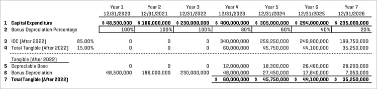
Finally, after 2022 a portion of the capital expenditure that represents tangible capital expenditure can still be deducted as bonus deprecation. For example, in 2023, if 85% of capital expenditure is deducted as IDCs, then 80% of the remaining 15% can be deducted as bonus depreciation, and the remainder counts toward the depreciable base which is depreciated over its useful life. Figure 1 shows how capital expenditure can be deducted as IDCs, depreciation, or bonus depreciation.
Figure 1. IDC, Depreciation and Bonus Depreciation Analysis
Depletion
Depletion is a form of depreciation for mineral resources that allows for a deduction from taxable income to reflect the declining production of reserves over time. As illustrated in Figure 2, under the units of production method, to estimate the depletion expense for Year 1, the production volume in Year 1 is subtracted from the total volume of reserves at the beginning of the projection period. This results in the ending reserve volume for Year 1. The ending reserve volume for a given year represents the beginning volume for the following year. The relationship between the production for a given year and the reserves volume at the beginning of that year implies the depletion rate. Multiplying the depletion rate for that year by the estimated value of the reserves results in the depletion expense for the year.[4] This process is repeated annually for the life of the reserves.
Figure 2. Depletion Analysis – Unit of Production
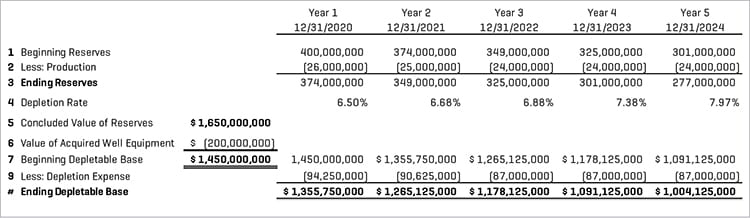
When an acquisition is structured as an asset transaction, the value of well equipment and machinery associated with the acquired oil and gas reserves can be immediately expensed. Therefore, this amount must be excluded from the value of the oil and gas reserves when calculating the depletion expense, as shown above.
Subtracting G&A expense, depreciation, bonus depreciation, depletion, and IDCs from the operating cash flow results in the acquired properties’ taxable income, before the consideration of net operating losses (NOLs).
Net Operating Losses
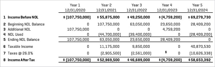
Before the TCJA was passed, taxpayers were permit¬ted to carry back NOLs two years and carry forward NOLs 20 years to offset taxable income in such years. However, the TCJA eliminated taxpayers’ ability to carry back NOLs arising after 2017 and removed the 20-year expiration period, but allows all NOLs to be carried forward indefinitely and limits the annual NOL deduction to 80% of taxable income.[5] However, the TCJA allows NOLs arising in 2017 and before to be carried forward without the 80% limitation. Because acquisitions of oil and gas properties are structured as asset transactions, no historical NOLs are assumed to be included with the acquired properties. Therefore, the beginning NOL balance is typically zero. Figure 3 is a simple illustration of the determination of NOLs.
Subtracting the NOLs used, if any, from the income before NOL results in taxable income.
Figure 3. Net Operating Losses and Taxable Income
Income Tax Rate
The income tax rate applied to taxable income varies widely based on the location and the tax history of the acquirer. The acquirer’s tax department can estimate what appropriate effective tax rate should be used. For simplicity, the tax department can use the sum of the federal and state corporate tax rate (21% + state tax rate).
Multiplying the tax rate by the taxable income results in the annual income tax expense. Subtracting the income tax expense from the income before NOL results in the income after tax.
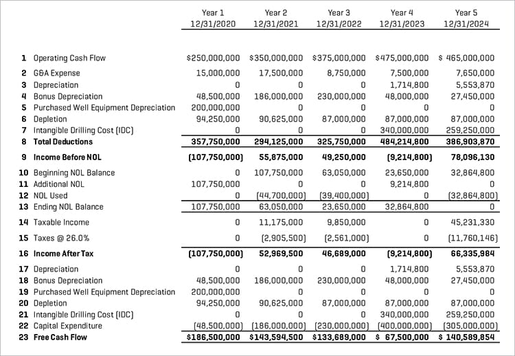
Free Cash Flow
As shown in Figure 4, the final steps in estimating the free cash flow of the acquired oil and gas properties involves the following adjustments to income after tax. Depreciation, bonus depreciation, the value of well equipment and machinery associated with the acquired oil and gas reserves, depletion, and IDCs are added back, because these expenses do not reflect actual cash outflow of the acquired properties but were deducted to determine the taxable income. Finally, cash outflows associated with expected capital expenditures are subtracted because these amounts have not yet been reflected in the projected cash flows.
Figure 4. Free Cash Flow
The resulting post-acquisition free cash flows of the acquired properties can then be used for internal budgeting or in valuations under fair value accounting. Using these projected free cash flows in a discounted cash flow analysis, discounted at an appropriate discount rate, analysts can conclude the value of the acquired oil and gas properties.
- For fair value accounting of oil and gas properties, we typically assume an asset transaction, even if the deal was structured as a stock transaction.
- For simplicity, we exclude natural gas liquids (NGLs) from the discussions; however, NGLs can be included in the acquired properties.
- The first three years of NYMEX contracts are the most liquid, and therefore, we believe they provide more meaningful indications of future prices. The further out you go, the less liquid the market and the less relevant the market data.
- The value of the reserves is ultimately based on the projected cash flow of the properties, which is affected by the depletion expense. Thus, this creates a circular or iterative process that can be solved with a spreadsheet or financial model.
- Pursuant to the Coronavirus Aid, Relief, and Economic Security Act (the CARES Act) effective March 27, 2020, the 80% statutory limitation was temporarily removed. In addition, firms may take NOLs earned in 2018, 2019, or 2020 and carry back those losses five years.