Valuing early stage, technology-based intellectual property assets is challenging, in large part due to the difficulty in incorporating the effects of risk and uncertainty inherent in these assets into their valuation. Monte Carlo methods were originally designed to model physical and mathematical problems. However, variations of this method also provide valuation analysts with a powerful tool to effectively address risk and uncertainty, particularly in the context of determining intellectual property values related to transactions or strategic decision-making.

The challenge of assessing and incorporating risk into various methods used for valuing intellectual property

Technology-based intellectual property (“IP”) assets, usually protected as patents and/or trade secrets, are typically valued using the same three common approaches as are used to value businesses or other assets. These approaches include, 1) income approach,¹ 2) market approach,² and 3) cost approach.³ However, technology-based IP assets (and many other IP assets including patents and trade secrets unrelated to technology, along with trademarks and copyrights) pose many unique challenges to a valuation analyst. A few illustrative examples of such challenges include:

• Income approaches are often difficult to implement for a variety of reasons, including the difficulty in quantifying the portion of a product or service’s cash flows that are attributable to the subject IP asset.
• Market approaches are often difficult to implement for many reasons, including the fact that IP assets are, by definition, unique. As such, comparable market transactions are often difficult or impossible to find. In addition, because IP assets are not traded on public markets and the transactions themselves are typically confidential, there are few public sources that reveal deal details that would be sufficiently comparable to be used to implement a market approach, and the data available from sources that do exist is often incomplete.
• Cost approaches are often difficult to implement because the cost to create the subject assets is almost always unrelated to the value of the asset (e.g., income generation, cost savings, etc.) that can be gained from use of the asset.

However, in addition to these challenges, perhaps the most difficult issue associated with valuing technology-based IP assets is accounting for the significant risks associated with many of these assets. Accounting for risk is particularly difficult in the very common situation when technology-based IP assets are valued prior to any (or significant) commercialization success; i.e., when the assets are “early stage.”

Early stage, technology-based IP assets are inherently risky for a variety of reasons, including, but not limited to:

• Claims included in the patent applications may not survive to the issued patents and the scope of surviving claims may be uncertain
• Issued patents may prove to be invalid when challenged
• Trade secret protections are not guaranteed
• Successful completion of an in-process technology is not guaranteed
• Implementation of the subject technology into products and services may be difficult or impossible
• Manufacturing scale-up may not be technically viable
• Costs of R&D, product integration, and manufacturing scale-up may be much higher than anticipated, perhaps even prohibitively high
• Market success has not been convincingly proven and often cannot even be tested until late in the product development process
• Anticipated regulatory approvals may be delayed or denied
• Unanticipated safety and efficacy issues may arise related to the in process or finished product
• Non-infringing alternatives to the subject assets or design-around options may be difficult to identify and assess
• Innovation may be moving at a rapid pace, causing the economic life of a particular technology to be unknown and, perhaps, short-lived

Risk and uncertainty associated with early stage, technology-based IP assets can be addressed by the valuation analyst through a number of methods, including:

• Performing significant due diligence to identify, understand, and assess the various areas of risk and uncertainty
• When using an income approach, adjusting the discount rate used as part of a discounted cash flow (“DCF”) model upward to reflect the identified and assessed risks⁴
• Using sensitivity analysis to understand the effect on value from changing certain variables
• Developing various scenarios (best, likely, worst case, etc.)
• Implementing decision-tree analysis
• Using option pricing techniques

In addition to these and other methods, the use of Monte Carlo simulations in conjunction with the Income Approach provides the valuation analyst with a flexible, powerful tool for performing valuations of early stage, technology-based IP assets. Given the nature of Monte Carlo simulations, they are particularly useful when the valuation is being performed to support transactions or strategic decision-making.

An explanation of the Monte Carlo method

The Monte Carlo method is a probabilistic technique that allows the analyst to run many “what-if” scenarios to arrive at a probability-weighted distribution of possible asset values rather than arriving at a single value as is the case for many other valuation methods. The Monte Carlo method is most often used in conjunction with the application of an Income Approach to valuing early stage, technology-based IP assets. Compared to a traditional DCF model that generates a single net present value (“NPV”) result, the Monte Carlo model, available through various software programs and Microsoft Excel plug-ins, gives the user the flexibility to assign various probability distributions to key assumptions and run a large number of trials to determine a distribution of NPVs based on the variability assigned to key assumptions. In doing so, the users of the model are able to better account for the inherent uncertainty in predicting the future value of key assumptions and, therefore, provide a more holistic look at the potential value of relevant IP assets.

As mentioned earlier, estimating the value of early stage, technology-based IP assets often involves a considerable degree of uncertainty, given the vast number of possible values of many of the key assumptions that can affect a DCF model. As one example, an estimate of total future research and development (“R&D”) costs expected to be incurred to complete or implement an in-process technology, and the timing of such expenditures, could vary significantly as of the date of the valuation. The Monte Carlo method allows the analyst to account for this inherent uncertainty of values related to key DCF assumptions in the model by assigning 1) various potential values, or a range of values, for each relevant assumption/variable and 2) a probability distribution of varying types. The DCF model can then be run multiple times to generate a range of potential values using these different potential inputs. It is not uncommon to run tens of thousands of trials, if not more, to generate an accurate distribution of possible NPVs. Essentially, the program is simulating all the possible NPV outcomes, given the variables, variable ranges, linkages between the variables, and distributions of these variables provided by the valuation analyst.

Many assumptions are used when valuing early stage, technology-based IP assets. When using the Monte Carlo method, the user has the capability to decide whether each assumption is a single value or whether it would be best to use a probability distribution to assign a range of values to an assumption. The type of probability distribution assigned to the assumptions are flexible in that the user can define the type and shape of the distribution5 along with the mean, standard deviation, and any upper or lower bounds. For instance, one of the reasons we decided to use the Monte Carlo method in the example we describe later in this article was the significant variability of the possible outcomes from our key value drivers.

Some of the variables and related potential outcomes were discreet such as, “Will the product receive U.S. Food and Drug Administration (“FDA”) approval? The answer to this question would be a simple “yes” or “no” with assigned ranges of probabilities associated with each. However, other variables had three or four possible outcomes with differing probabilities of occurrence. In addition, other variables had continuous distributions of various kinds, such as a “normal” or “Pareto” distributions.

Once all variables have been identified and their ranges and probability distributions selected, the valuation analyst can perform many “runs” of the model to determine the resulting unique NPV. For each “run” the software selects a specific value for each of the variables based upon the range, distribution, and probability of outcomes provided for each variable. The distribution of possible NPVs, or outcomes, generated as a result of running the DCF model many, many times with various combinations of values for the variables provides a probability-weighted range of NPV outcomes accurately reflecting the myriad combinations of the ranges, distributions, and probabilities input for each the key variables.

As mentioned earlier, risk and uncertainty are often addressed in a DCF model through the determination of a single, appropriate discount rate. However, when dealing with early stage, technology-based IP assets, this approach may have certain challenges. In particular, by compressing many individual risk elements into one discount rate, the analyst may be challenged to focus on and evaluate any one individual risk when the risks are many and the future is very uncertain. An advantage of the Monte Carlo method is that it allows the valuation analyst to shift the recognition of risk and uncertainty away from the discount rate to the cash flow projections. This is an advantage because the specific risks formerly bundled together in the discount rate can be much more closely analyzed and quantified through their effect on the NPV of projected future cash flows. Especially where there is great uncertainty and complexity, the Monte Carlo method allows the user to explicitly model the distribution of risks around key value drivers based on the best current information and expectations. The software performs the tens of thousands of computations necessary to model the interactions of the various key variables into a resulting range of probability-adjusted NPV outcomes. As a result, the Monte Carlo method allows the valuation analyst to visualize and make statistical statements around various predicted outcomes of the DCF model.

A Case Study for the Application of the Monte Carlo Method

By way of illustration, we present below an example of one of our actual applications of the Monte Carlo method.

We were asked to assist a medium-sized medical device company – “ExampleCo” – in its evaluation of the possible introduction of a new, patent-protected, cutting-edge medical device. Introduction of this product was capital intensive, requiring substantial long-term expenditures in R&D as well as investment in a capital-intensive manufacturing process. At the date of the valuation, investment-to-date was over $150 million and prospective investment was expected to be another $100 million. This investment was viewed by our client’s management and their board of directors as a “bet the company” decision and they invited us in to help them to research, evaluate, and model their options so that they could make a wellinformed decision regarding how to proceed with the project.

The company was facing substantial uncertainties on many fronts related to its prospective new product. To name but a few, it was facing such issues as:

• Its ability to complete the product and make it function properly
• Its ability to complete the project on time and on budget
• Market acceptance and the level of worldwide demand for its product
• The extent of cannibalization of its own existing products by the new product
• Emerging competing products and technologies
• Regulatory acceptance such as FDA approval
• Reimbursement under federal medical insurance programs
• Eligibility for, and rate of reimbursement under, medical insurance coverage

Initially, we created a traditional multi-year DCF model addressing issues such as sales revenues, services revenues, costs of goods sold (“COGS”), service and warrants costs, selling, general and administrative (“SG&A”) costs, royalties payable,7 development costs, taxes, and other cost items specific to the new product introduction. When completed, this model provided us with a “point-estimate” of the IP embodied in the new product under development. In this initial valuation analysis, all of the risk and uncertainty associated with the values of each of these variables was incorporated into the discount rate used to discount future cash flows to the present in the form of an NPV. Because risks associated with many or all of the variables were pervasive, complex, and/or interactive among the variables, we decided to use the Monte Carlo method. We took advantage of the initial DCF analysis that generated the “point estimate” and used it as the base upon which we built the Monte Carlo simulation.

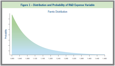
As an early step in the process, we described the expected range of possible outcomes and the expected “shape” of the distribution of the reasonably possible outcomes associated with the key value drivers. See Figure 1 below as an illustration of assigning a distribution to a value driver. This figure represents the distribution of outcomes and their related probabilities associated with total R&D costs. The graph depicts a Pareto distribution of outcomes, with a 50 percent probability that the total R&D costs would finish on budget (we assigned no chance that the new product research would be completed under budget) and generally diminishing probabilities of overrun amounts up to approximately a maximum 50 percent overrun of the R&D budget. Our R&D cost estimation was informed by discussions with the project leaders, study of the client’s similar prior projects, and identification and examination of competitors’ comparable projects.

After following a similar process of assigning low and high values and distributions to the other value drivers, we proceeded to run the DCF model using the Monte Carlo tool for individual lines on the cash flow forecast such as price per unit, unit sales, COGS, and SG&A expenses. This intermediate step was performed to, 1) understand how these revenue or cost items were behaving based on the modeled distributions and linkages between variables, and 2) determine the relative effect of the individual value drivers within each revenue or cost category. For instance, Figure 2, shows an illustrative distribution of unit sales in thousands.

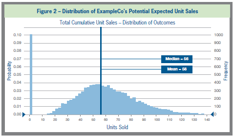
After the DCF model was run through the Monte Carlo simulator 10,000 times, the unit sales summary variable had the distribution shown in Figure 2. The distribution of results ranges from 0 units sold to almost 140,000 units sold. As can be seen from the figure, this distribution turned out to resemble a “normal” distribution with, 1) an outlier probability of 10 percent that there would be zero units sold, and 2) a slight skew toward the higher-value side of the distribution. In this example, both the mean and median was 56,000 units sold as indicated by the tall dark blue bar. The other tall bar at zero units sold represents our judgment that there was a 10 percent chance that the project would fail and, as a result, never produce any commercial sales.

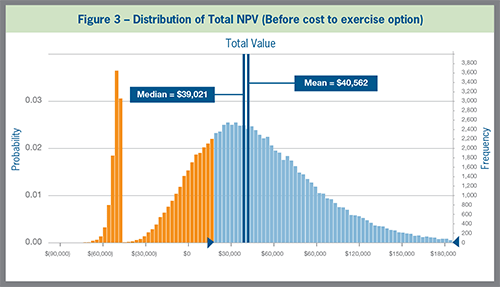
When all variables were combined, our total project NPV estimate looked like the distribution shown in Figure 3, which portrays the results of 100,000 separate simulations of the project’s results for the company. As can be seen, the project’s distribution of NPV results is still approximately a “normal” distribution skewed slightly to the higher project values with an offsetting pillar of negative NPV outcomes assuming project failure and zero commercial sales. The mean of the distribution is $40.6 million and the median is $39.0 million. The point where the bars change in color from orange to blue represents the NPV at which the client determined a go/no-go decision would be made.

This ability to visualize and make statistically valid statements regarding the results of the analysis is one of the key advantages of using the Monte Carlo method over point-estimation techniques. Another major advantage is the unbundling of risk adjustments from residing solely in the discount rate. In fact, in this instance, we reduced the discount rate we used when implementing the Monte Carlo method from over 40 percent that was used in the initial DCF model that generated a point-estimate NPV to just above 12 percent in our Monte Carlo analysis.⁸

As an illustration of the modeling capabilities of the Monte Carlo software we used, note that the zerovalue results in Figure 3 do not look the same as the zero units bar in Figure 2. The reason is that we modeled that the “no-go” decision could be made at different times after differing types and amounts of investments; hence there are different levels of losses associated with the different dates at which the project might be terminated. Figure 3 also shows that there is some possibility that the new product may actually enter production but never make it to profitable levels. On the other hand, the graphic in Figure 3 demonstrates that there is almost a 5 percent chance of NPV results in excess of $120 million.

In this article we introduced the Monte Carlo method, one of several commonly used financial modeling tools employed by IP valuation analysts. The Monte Carlo method is particularly effective when used to determine the value of early stage, technology-based IP assets and is well suited to address valuation issues in the context of transactions and strategic decision-making. However, compared to the use of many other valuation tools, implementation of the Monte Carlo method has certain challenges.

For instance, use of the Monte Carlo method can involve some initial investment of time devoted to understanding the technique and related software. In addition, the use of the technique often requires additional time not necessarily required of other methods to model the variables and to perform due diligence to support the more detailed modeling. Consequently, it is prudent for the analyst to carefully evaluate each particular valuation opportunity in light of the particular costs and benefits associated with the Monte Carlo method before making the choice to use this method. With that said, it has been the authors’ experience that if the choice is made to invest in the Monte Carlo method, the analyst is typically rewarded with insightful and intuitive outputs accurately reflecting the various risks associated with the IP being valued.

---

¹ Per the International Glossary of Business Valuation Terms, Appendix B to the Statement on Standards for Valuation Services (“SSVS”) promulgated by the American Institute of Certified Public Accountants (“AICPA”), the income approach is defined as “a general way of determining a value indication of a business, business ownership interest, security or intangible asset using one or more methods that convert anticipated economic benefits into a present single amount.”
² Per the International Glossary of Business Valuation Terms, Appendix B to the SSVS romulgated by the AICPA, the market approach is defined as “a general way of determining a value indication of a business, business ownership interest, security or intangible asset by using one or more methods that compare the subject to similar businesses, business ownership interests, securities or intangible assets that have been sold.”
³ Per the International Glossary of Business Valuation Terms, Appendix B to the SSVS promulgated by the AICPA, the cost approach is defined as “a general way of determining a value indication of an individual asset by quantifying the amount of money required to replace the future service capability of that asset.”
⁴ From our experience, and supported by various third parties, discount rates used in conjunction with discounted cash flow models for valuing early stage, technology-based intellectual property assets commonly range from 20 percent to 75 percent (and sometimes higher). This is in stark contrast to discount rates used, for example, when valuing businesses, which typically reflect the subject business’ weighted average cost of capital (“WACC”). Per Morningstar, as of December 31, 2012, the median WACC for a sampling of 381 large-capitalization companies was 7.73 percent.
⁵ Illustrative standard distribution types that can be used include: Normal, Triangular, Uniform, Lognormal, Beta, Gamma, Exponential, Pareto, Poisson, etc. In addition, the valuation analyst can typically create his/her own custom distribution type.
⁶ Note that the facts and results regarding the project have been modified to preserve confidentiality.
⁷ Material royalties were payable on licensed technologies embedded in the products being introduced.
⁸ The rationale and mechanics underlying this reduction is beyond the scope of this article.